转自:[机器学习ML NOTE] CNN演化史(AlexNet、VGG、Inception、ResNet)+Keras Coding)
我这里只列出几个比较重要的突破,也是比较经典的模型。
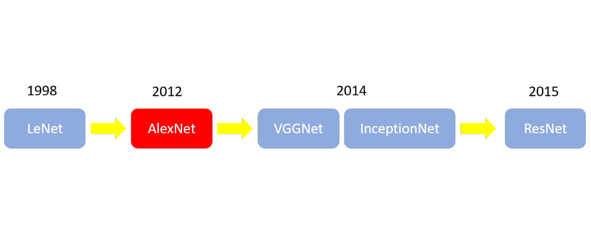
CNN Classification revolution
为什么AlexNet会标成红色呢?因为在2012年这一年中,AlexNet为一个重大的突破,也开始了大CNN时代,CNN开始有了很大的突破,各种CNN的模型也开始出现,也站稳了在影像上面很重要的一席之地,接下来我来简易介绍各种模型,然后也附上各种Model在分类上的实作(Keras)
LeNet(论文连结)
没错,这就是CNN之父,前面也介绍过了卷积跟池化,所以应该可以很容易理解LeNet的运作,就是简单利用了卷积跟池化,并接上全连结层做分类,这里我们用Mnist data来实作LeNet training
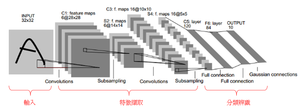
LeNet Architecture, 1998
1 | import numpy as np |
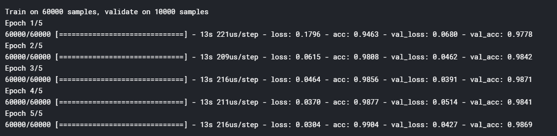
Train 5 个epoch就可以达到98.69的精确率
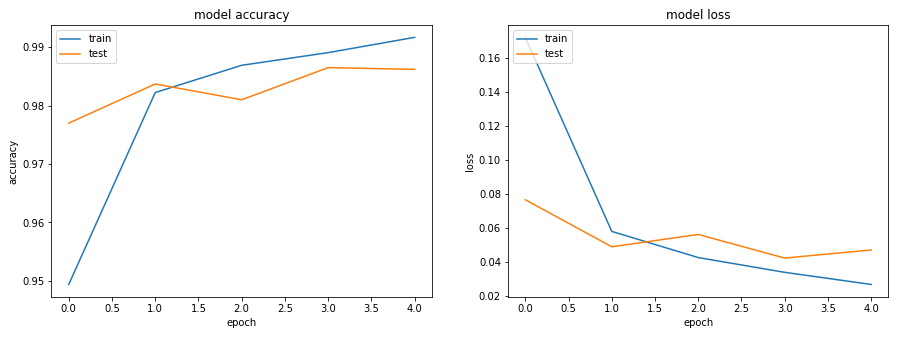
Loss 跟 Accuracy
AlexNet(论文连结)
AlexNet 在2012年的ImageNet LSVRC的比赛上拿了冠军,而且准确率完胜第二名,那时候造成很大的轰动,也使得CNN开始被重视,变成所谓的CNN大时代,之后的比赛也都是由CNN拿下冠军,深度学习正式大爆发。
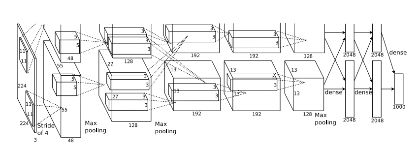
AlexNet structure
AlexNet的特点:
- 使用了非线性的激活函数(Activation function):Relu
对于什么是Activation function,我之后会找时间来介绍,不懂的可以先参考这个网站,在AlexNet以前,大部分的网路都是用tanh当作激活函数 - 使用了Data augmentation 和Dropout 来防止Overfitting
- 多个GPU并行运算
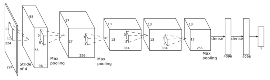
之所以为什么上面架构会分成上下2层去训练,是因为当初在训练的时候记忆体不够所以分成两块在GPU上训练,其实这样的网路要弄成一层也是可以的,以下这张图就是一层的网路架构图,其实是跟LeNet有点类似的,这里我用开源dataset oxflower17来实行AlexNet,我也加入了data augumentation,大家可以参考看看。
1 | import numpy as np |
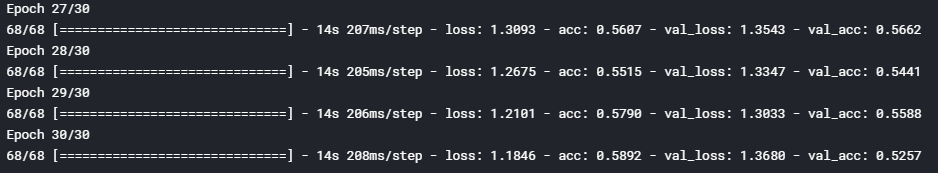
30个epochs可达到55% 准确值
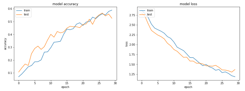
Loss and accuracy of AlexNet
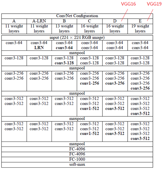
VGGNet(论文连结)
VGGNet在2014年ILSVRC的分类比赛中拿到了第二名(第一名是等等要介绍的InceptionNet),其实VGGNet跟AlexNet之间并没有什么太大的差异,只是将网路的深度变深,进而得到更好的结果,我一样用开源dataset oxflower17来实行VGG16Net,因为VGG16的深度变深,相对的,VGG的参数就会是AlexNet的好几倍,训练时间也会相对的较长。
1 | import numpy as np |
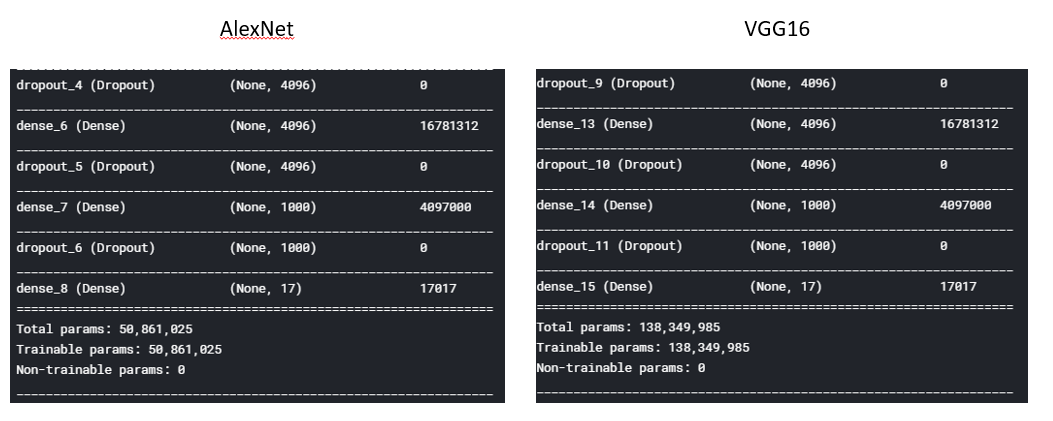
VGG16的参数量为AlexNet的3倍左右
Inception(GoogLeNet)
GoogLeNet在2014年ILSVRC的分类比赛中拿到了第一名,GoogLeNet做了一个创新,他并不是像VGG或是AlexNet那种加深网路的概念,而是加入了一个叫做Inception的结构来取代了原本单纯的卷积层(但他其实也是利用卷积来达成),而他的训练参数也比AlexNet少上好几倍,而且准确率相对更好,所以当时才拿下了第一名的宝座,一直到现在,Inception已经衍生到InceptionV4。
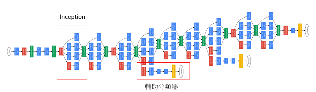
GoogLeNet 架构
而GoogLeNet最重要的就是Inception架构:
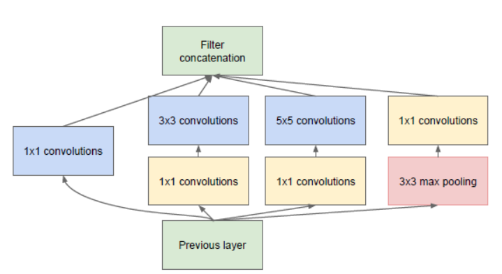
Inception架构
GoogLeNet将3种convolution跟一个pooling叠在一起,增加了网路的宽度,而且这样堆叠在一起后,更能撷取输入图片的更多的细节讯息跟特征,那为什么要加一个1x1的卷积呢?其实他的目前就在于减少图片的维度跟减少训练参数,假设我们input的大小为100x100x56,如果我们做一个有125个filter的5x5卷积层之后(stride = 1 , pad = 2),输出将为100x100x125 ,那么这个卷积层的参数就为5655125 = 175000,如果我们先经过28个filter的1x1的卷积,再经过有125个filter的5x5卷积层之后,输出一样为100x100x125,但是参数就减少成561128+2855*125=89068,相对少了快一半的参数。
GoogleNet有以下几种不同的地方:
- 将单纯的卷积层跟池化层改成Inception架构
- 最后分类时使用average pooling来替代了全连结层
- 网路加入了2个辅助分类器,为了避免梯度消失的情况
论文连结:
Inception V1 , Going Deeper withConvolutions.
Inception V2 , Batch Normalization:Accelerating Deep Network Training by Reducing Internal Covariate Shift.
Inception V3 ,Rethinking theInception Architecture for Computer Vision.
Inception V4 , Inception-v4,Inception-ResNet and the Impact of Residual Connections on Learning.
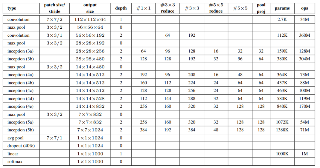
我们用InceptionV1论文中提到的这个Table来实现GoogLeNet的网路,跟之前一样,都用开源dataset oxflower17来进行训练,
1 | import numpy as np |
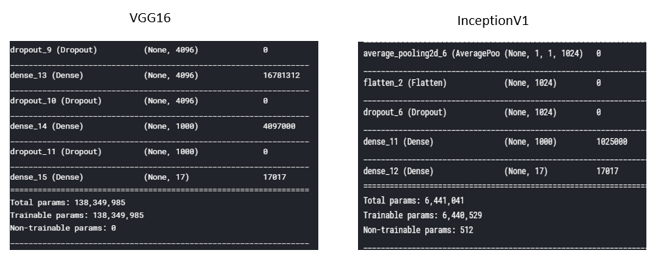
Inception的参数为VGG的1/20左右
ResNet残差网路(论文连结)
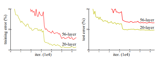
我们经过之前VGG的结果,深度学习是不是越深就越好呢?如果一直无限延伸的增加层数,是不是结果就会比较好呢?我们来看一下论文里面的图,咦!?怎么56层的网路结果却比20层的网路差!!!,不是说越深越好吗?
=======================================
在经过实验后发现:网路层数的增加可以有效的超加准确率没错,但如果到达一定的层数后,训练的准确率就会开始下降了,这代表说如果网路过深的话,会变得更加难以训练
=======================================
那为什么深度越深反而变得更难训练呢?我们回到神经网路反向传递的部份,我们知道要更新参数的方法是利用Loss function对参数的偏”微分”来得出参数调整的梯度,通过不断的训练,来找到一个Loss function最小的结果,如果现在是只有1层网路,反向传递的梯度也就只需要传递1次,相对的,如果现在有100层网路,反向传递的梯度就需要传递100才能到最前面的参数,所以当网路层数加深时,梯度在传递的过程中就会慢慢的消失,这也就是所谓的梯度消失,就会无法对前面网路层的参数进行有效的更新,因此Deep Residual Network就出现了,也就是ResNet。
PS想知道关于梯度消失和梯度爆炸的可以先参考这篇文章,写得很好。
深度残差网络参考你必须要知道CNN模型:ResNet
重点来了,什么是DRN呢?这边就有点小抽象了,可能需要想一下才会理解,我先把残差网路的架构图放上来
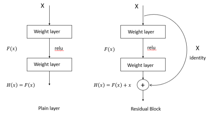
从上面图来看,左边是一般的网路(平原网路),右边是加入捷径的残差网路,我们假设H(x)是我们的期望输出,原本网路的最后的H(x)就是F(x),而我们可以看出在残差网路那边在F(x)加上了原本的输入x,所以H(x)=F(x)+x,那为什么要这样呢?
这里我们来思考一下,前面我们说到了反向传递,是用loss function来决定的,而loss function不外乎就是跟output跟target的值,然而我们说到了梯度消失的问题,假设我们已经学习到比较饱和的准确率的时候,那么接下来要学习的目标就会变成是”恒等映射”的学习,而什么是恒等映射呢?其实就是要将输入x 近似于输出H(x),这样就可以保持后面的层数中比较不会造成准确率下降。
好吧,或许你看到这里还是有些不懂,那我们来看一下右边的残差网路,残差网路在输出的部份加入了一个x,输出H(x)就会变成H(x )=F(x)+x,那如果我们把F(x)=0时,咦!?就会变成H(x) = x了,这不就是前面所说的恒等映射吗?所以残差网路就变成训练F(x):H(x)-x,而目标就是要将F(x)趋近于0,这样才可以使网路加深,准确率不会下降。
上面一堆文字你是不是快崩溃了,我自己在读的时候也是快崩溃了XDD,我想了一下,这是不是就跟”以讹传讹”这句成语是一样的意思呢?如果传的人越多,那错误率是不是就越高,而残差网路的捷径就是直接把话传给最后一个人来减少错误率(如果这想法有错请帮忙纠正><),大概就是下面这张图的概念XD

然后论文有说到优化残差网路比优化原本网路更好,这又是为什么?我直接来举个例子会比较好了解:
======================================= =
假设输入x = 5
经过第一层出来后的H(x)为5.1,那么F(x) = 5.1–5 = 0.1
经过第二层出来后的H(x)为5.2,那么F(x) = 5.2–5 = 0.2
原本网路的变化率会是(5.2–5.1)/5.1 = 1.96%
那残差网路的变化率是多少(0.2–0.1)/0.1 = 100%
对的,残差网路对于调整参数的效果会更好
残差去掉了相同的主体部份,进而突显出微小的变化================================== ======
终于把理念讲完了(头痛…),接下来我们来进行实作啦~~~~
我们来看一下论文上面的网路跟卷积核数量,我们会发现一件很奇怪的事,为什么残差网路的捷径有分实线跟虚线的部份,再仔细看一下,虚线的部份的输入channel跟中间的F(x)channel是不一样的,所以虚线的部份会再对输入x进行一次卷积来调整x的维度再进行相加=> H(x)=F(x )+Wx,W就是卷积。我们直接上Code啦(实作ResNet34)!
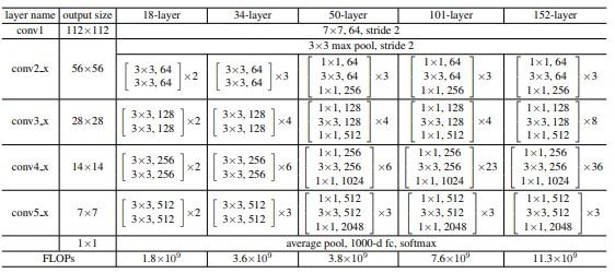
1 | import numpy as np |
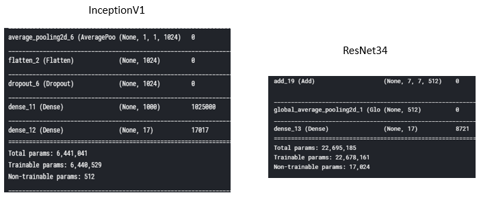
参数量比Inception多
结论
最后附上全部Model的Github,CNN的演进是很有趣的,有些观念其实还满直观的,只是就是想不出来,这些演进大多都是基于最基本的卷积跟池化演变来的,之后还有一些CNN的变形,Attention,RCNN…等等等的CNN模型用在影像处理上面,不得不说,CNN真的是太有趣了